Basic HTML Version


International Journal of Marine Science 2014, Vol.4, No.42, 1-11
http://ijms.biopublisher.ca
6
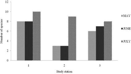
Figure 5 Variations in the number of benthic macroinvertebrtae
species recorded at the study stations during the wet season.
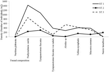
Analysis of the spatial occurrence of the species
observed (Figure 6) indicates that only six spp (
P.
aurita, T. fuscatus, T. fuscata
var
. radula, Aloides
sp.,
T.
nymphalis, M. cumana
) occurred in all the study
stations.
Nereis lamellose
was restricted to stations 1
and 2, while
Neritina glabarata
occurred only in
station 1. All the species recorded highest densities in
station 1 (except
N. lamellose
which occurred in
greatest number in station 2). Generally, individual
species representation was lowest in station 2.
Although, differences in spatial distribution were clearly
evident, that cannot be said of the seasonal density.
Figure 6 Spatial variation in density of benthic
macroinvertebrate species
2.4 Structure of functional feeding groups (FFGs)
Analysis of the functional feeding composition of the
macroinvertebrate assemblage revealed that, of the
two FFGs (Table 2) recorded, filter feeder was the
most abundant FFG, it accounted for 67.4 % of the
total benthic macoinvertebrate population, while the
deposit feeders constituted 30.05 %. A predatory
species
Nereis lamellose
which constituted 2.56 % of
the total population was recorded. The population of
the filter feeders was dominated by the gastropod
P.
aurita
, which accounted for approximately 48 % of
the observed population; this was followed by
T.
nymphalis
which constituted 18.78 %.
Table 2 Faunal composition and feeding groups
Taxa
Functional feeding group
Bivalva
Aloididae
Filter feeder
Arcidae
Filter feeder
Ostreidae
Filter feeder
Gastropoda
Melaniidae
Filter feeder
Potamididae
Deposit feeder
Polycheata
Nereididae
Predators/scavengers
Filter feeders were recorded in all the study stations,
however,
N. glabarata
was absent in stations 2 and 3,
and the predator was not recorded in station 3.
Densities of filter and deposit feeders were highest in
station 1, while that of the predator was highest in
station 2.
2.5 Spatial temporal variations in primary productivity
The concentrations of chl-a in surface water and
sediment of the study area are presented in Table 3,
while Figures 7~11 illustrate its spatial and temporal
variations during the study period. Generally, values
of chl-a were higher in water samples than in sediment.
The amount of chl-a in water was highest (5.06 mg/L)
in the month of March and lowest (0.9 mg/L) in the
month of February. Total chl-a values recorded for the
other sampling months were; 2.47 mg/L in July,
2.43 mg/L in June, 2.15 mg/L in May and 2.06 mg/L
in April. The concentrations of chl-a in water during
the study months were significantly different
(ANOVA, F = 8.883,
p <
0.05), a
post-hoc
test using
Turkey’s Test shows that values of chl-a were
significantly lower in the month of February and
significantly highest in the month of March, while
values recorded for the months of April, May, June
and July were similar. Monthly values varied between
0.12 – 0.46 mg/L in February, 1.13 – 2.01 mg/L in
March, 0.53 – 0.89 mg/L in April, 0.57 – 0.89 mg/L
May, 0.61 – 0.98 mg/L in June, and 0.53 – 1.01 mg/L
in July. There was variation in values of chl-a
recorded in the study stations, although values were
not significantly different (ANOVA, F = 0.005,
p >
0.05). Total concentration of chl-a in water was
highest in station 1 and lowest in station 2.