Basic HTML Version


International Journal of Marine Science 2014, Vol.4, No.61, 1-13
http://ijms.biopublisher.ca
5
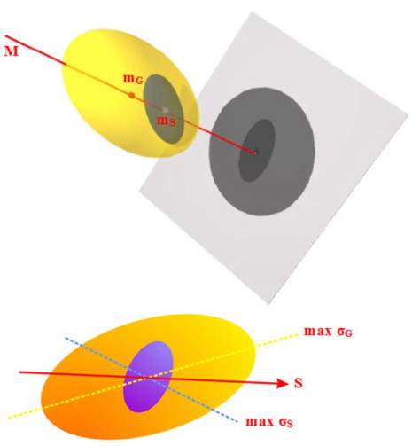
Figure 2 Geometric interpretation of ENFA: Large gray circles
represented the entire cell space (global), while the smaller
dark circles represented parts of the cells of studied species.
Straight line passing through the midpoint of the two spaces
(m
G
and m
S
) was the marginality factor (M), while the
specialization factor (S) was the axis maximizing the ratio of
the global variance (σ
G
) with variance species (σ
S
), which was
the mean value of maximum global variance with a minimum
species variance (Modified from Hirzel et al., 2002)
The area-adjusted frequency of cells falling into each
bin range can then be computed as Fi=Ni/Ai. A
completely random map would result in Fi≈1 for each
bin range. A good fit of the data to the model is
indicated by a low Fi for low HS values and a high Fi
for high HS values (Hirzel et al., 2006). Range of
habitat suitability scale in this study was divided into
three classes according to Compton (2004):
Suitable habitat, the habitat suitability valued between
67 and 100.
Marginal habitat, the habitat suitability valued
between 34 and 66.
Unsuitable habitat, the habitat suitability valued
between 0 and 33.
Evaluation/validation of habitat suitability models
along with the data was using Area Under
receiver-operating-characteristic Curve (AUC). This
validation technique was cross-validation with
presence-absence data to assess the accuracy of the
ENFA model. The relevant techniques were used, if
the species absence data was sufficiently reliable.
AUC values ranged from 0 to 1 with values close to 1
indicated a very good accuracy from the model (Hirzel
et al., 2006). Evaluation of both models with
continuous Boyce index method and the AUC had
also been integrated in the program BioMapper, so the
results could be seen directly from the program output.
Furthermore, to determine whether there were
differences in each environmental variable occupied
by scallop with the overall study area, then the
chi-square test was applied (χ
2
). If the data
characteristics did not allow for the chi-square test to
be conducted, then the Kolmogorov-Smirnov test
became the alternative. Range of values for each
environmental variable was divided into classes with
same interval. By using the ArcGIS, the location
frequency (grid) in each class was calculated both for
environmental variable from the entire study area and
the location frequency (grid) where scallop located
(Leverette, 2004).
2 Results
2.1 Characteristics of Scallop Habitat Environmental
Nine characteristics of environmental (eco-geographical)
variables which determined the scallop habitat were
presented in Figure 3, while the distribution of scallop
in classes in each of these variables was presented in
Figure 4.
Distribution of scallop at the study area based on the
eco-geographical variable was seabed with high
density of plankton (11,001-14,500 ind/L), between
18-31 m water depth, low TSS (< 3.61 mg/L), soft
sediments (mud, φ ≥ 6) and a relative distant from
estuary (> 5 km). In addition, the scallop also required
benthic habitat with high current velocity and salinity
(> 0.06 m/sec; 31.85-32.65 ‰) and relatively low
temperature (29.92-30.06 °C). Meanwhile, scallops
were relatively more tolerant to the pH (7.3-7.4).
2.2 Suitability and Potential Habitat of Scallop
Ecological Niche Factor Analysis using 5 eco-
geographical variables showed Total Marginality
value of 1.069 (Table 2), indicating that the scallop
required habitats with very different conditions from
the mean habitat conditions existing throughout the
study area. Scallop habitat in the study area was largely

