Basic HTML Version


International Journal of Marine Science 2014, Vol.4, No.61, 1-13
http://ijms.biopublisher.ca
4
global mean and the mean of each species to
environmental variables (Hirzel et al., 2002),
calculated with the Equation (1).
………………… (1)
M = marginality
m
G
= global mean (study area)
m
S
= species mean
σ
G
= standard deviation of the global distribution
By combining the marginality coefficient of each
environmental variable, then ENFA calculated the
coefficient of Total Marginality (M
T
) (Hirzel et al.,
2002), represented with Equation (2).
.………………... (2)
V = number of environmental variables
m
i
= marginality coefficient of an environment
variable i.
The second and following components were species
specialization factors indicating how limited the
ecological niches of species was related to the study
area. The higher value of specialization in an
environmental variable indicated that the species
required a narrow range of environmental variables.
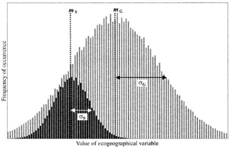
Its value defined as the ratio of the global distribution
of the variance species of environmental variables
(Figure 1, 2) (Hirzel et al., 2002) and calculated by
Equation (3).
…….…………………. (3)
S = specialization for an environmental variable
σ
G
= standard deviation of the global distribution
σ
S
= standard deviation of the species distribution
Analog to the Total Marginality, Total Specialization
coefficient (S
T
) could also be calculated by combining
the specialization coefficient of each environmental
variable and calculated with Equation (4).
Figure 1 The distribution of the focal species on any
eco-geographical variable (black bars) may differ from that of
the whole set of cells (gray bars) with respect to its mean (m
S
≠
m
G
), thus allowing marginality to be defined. It may also differ
with respect to standard deviations (σs ≠ σ
G
), thus allowing
specialization to be defined (Hirzel et al., 2002)
………………….. (4)
V = number of environmental variables
λ
i
= specialization coefficient of an environmental
variable i.
Total Tolerance coefficient, opposed to the Total
Specialization coefficient (1/S
T
), ranged from 0-1,
where the higher coefficient indicated the more
extensive ecological niches of species. In other words,
species were more tolerant to the environmental
variables. Marginality and specialization coefficients
would be calculated directly by BioMapper program.
The output of this program generated habitat suitability
maps of scallop accompanied with the factors analysis
explaining the role of environmental variables in
determining the suitability of seabed habitat.
In order to assess the ENFA model ability to generate
habitat suitability map, Continuous Boyce Index was
applied to evaluate the model (Hirzel et al., 2006)
which was a cross-validation with presence-only data.
Species availability data were divided into 10 parts of
the same data sets. Nine of the 10 data sets used to
calibrate habitat suitability maps, while the remaining
1 dataset used for validating the results. This
procedure was repeated 10 times. From the ten subsets
the number of cells which fall into a set number of HS
value bin ranges was calculated. Each bin covers a
portion of the maps area (Ai), and contains some
proportion of the validation cells (Ni).
G
S
G
.
m m
M
96 1
96 1
1
2
.
m
M
V
i
i
T
V
S
V
i
i
T
1
S
G
S

