Rice Genomics and Genetics - page 7

Rice Genomics and Genetics 2015, Vol.6, No.5, 1-10
http://rgg.biopublisher.ca
4
∆݌௧ ൌ ߙ ൅ ߩߚ௧ିଵ ൅ ߛܶ ൅ ∑ ߜ௞ ∆݌௧ି௞ ൅ ߤ௧ ௡௞ୀଵ
(1)
Here, ݌௧ is the rice price series being investigated for
stationarity, ∆ is first difference operator, ܶ is time
trend variable, ߤ௧ represents zero-mean, serially
uncorrelated, random disturbances, k is the lag length;,ߚ ,ߙ ߛ ܽ݊݀ ߜ௞ are the coefficient vectors. Unit
root tests were conducted on the ߚ parameters to
determine whether or not each of the series is more
closely identified as being I(1) or I(0) process. The
test statistics is the t statistics for ߚ . The test of the
null hypothesis of equation (1) shows the existence of
a unit root when ߚ ൌ 1 against alternative
hypothesis of no unit root when ߚ ≠ 1. The null
hypothesis of non-stationarity is rejected when the
absolute value of the test statistics is greater than the
critical value. When ݌௧ is non-stationary, it is then
examined whether or not the first difference of ݌௧ is
stationary (i.e. to test ∆݌௧ି ∆݌௧ିଵ~ I(1) by
repeating the above procedure until the data were
transformed to induce stationarity.
The Philips-Perron (PP) test is similar to the ADF test.
PP test was conducted because the ADF test loses its
power for sufficiently large values of “k” which is the
number of lags (Ghosh et al., 1999). It includes an
automatic correction to the Dickey-Fuller process for
auto-correlated residuals (Brooks, 2008, Mafimisebi
and Thompson, 2012). The regression is as follows:ݕ௧ ܾ଴ ൅ ܾଵݕ௧ିଵ ൅ ߤ௧ (2)
Where ݕ௧ is rice price series being investigated for
stationarity, ܾ଴ and b1 are the coefficient vectors ܽ݊݀ ߤ௧ is serially correlated error term.
3.2.3. Testing for Johansen Co-integration (Trace
and Eigenvalue tests)
If two series are individually stationary at same order,
the Johansen and Juselius (1990) and Juselius (2006)
approach can be used to estimate the long run
co-integrating vector from a Vector Auto Regression
(VAR) model of the form:∆௣೟ ୀఈା ∑ Г݅ ௞ିଵ ௜ୀଵ ∆݌௧ିଵ ൅ Π݌௧ିଵ ൅ ߤ௧ (3)
Where ݌௧ is a nx1vector containing the series of
interest (rice price series) at time (t), ∆ is the first
difference operator, Г݅ and Π are nxn matrix of
parameters on the ith and kth lag of ݌௧, Г݅ ൌ
൫∑ ܣ௜ ௞ ௜ୀଵ ൯ ₋ ܫ௚ , Π ൌ ൫∑ ܣ௜ ௞ ௜ୀଵ ൯ ₋ ܫ௚ , Ig is the
identity matrix of dimension g, is constant term,ߤ௧ is nx1 vector of white noise errors. Throughout, p
is restricted to be (at most) integrated of order one,
denoted I(1), where I(j) variable requires jth
differencing to make it stationary. Equation (2) tests
the co-integrating relationship between stationary
series. Johansen and Juselius (1990) and Juselius
(2006) derived two maximum likelihood statistics for
testing the rank of Π, and for identifying possible
co-integration as the following equations show:
λ௧௥௔௖௘ ሺݎሻ ൌ െܶ ∑ ܫ ݊ሺ1 െ ௠௜ୀ௥ାଵ λ௜ሻ (4)
λ௠௔௫ ሺݎ ,ݎ ൅ 1ሻ ൌ െܶInሺ1 െ λ௥ାଵ ሻ (5)
Where r is the number of co-integration pair-wise
vector, λ௜ is the eigenvalue’s value of matrix Π. ܶ is
the number of observations. The λ௧௥௔௖௘ is not a
dependent test, but a series of tests corresponding to
different ݎ values. The λ௠௔௫ tests each eigenvalue
separately. The null hypothesis of the two statistical
tests is that there is existence of r co-integration
relations while the alternative hypothesis is that there
is existence of more than r co-integration relations. In
this study, this model was used to test for; (1)
integration between pair-wise price series in any two
contiguous markets in the zone and (2) integration
among the six price series taken together.
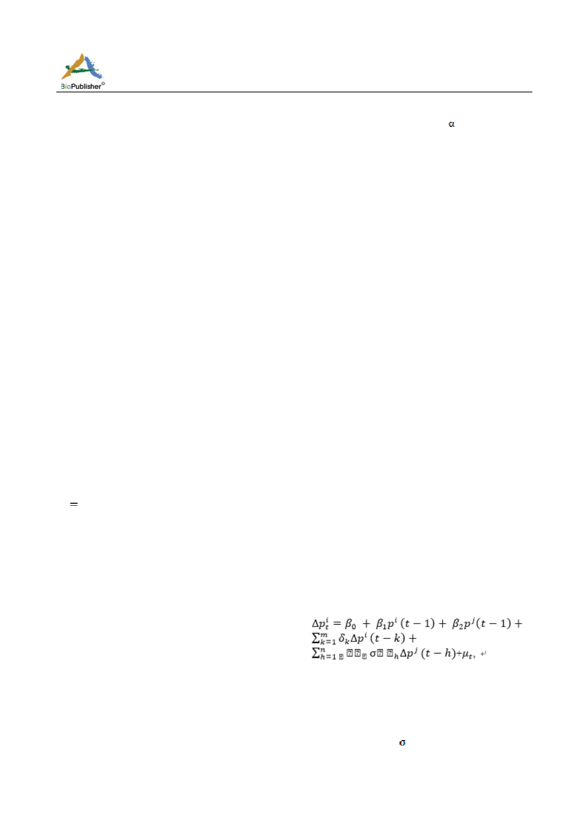
3.2.4. Test for Granger-causality
After undertaking co-integration analysis of the long
run linkages of the various market pairs, and having
identified the market pair that were linked, an analysis
of statistical causation was conducted. The causality
test used an error correction model (ECM) of the
following form;
Where, m and n are number of lags as determined by
Akaike Information Criterion (AIC).
Rejection of the null hypothesis i.e. that prices in
market j does not Granger cause prices in market i (by
a suitable F-test) for h = 0 for h = 1, 2 ….n and ߚ =0 indicated that prices in market j Granger-caused