International Journal of Horticulture, 2017,Vol.7, No. 23, 205-218
216
We plot a three dimensional figure on rate vs. time and seed weight in Figure 11. Recall the construction of
Figure 2, consider a fixed seed weight and consider the relevant plants with yam cut at the time of second interim
growth recording. For plants with a fixed seed weight,
y
co-ordinate of curves over different time points
x
,
whenever at least one data point from first interim, second interim, final harvest are available in a curve, that time
point was considered in Figure 2. Now for a fixed seed weight, compile all these time points, counted from the
time of sprouting in relevant plant, where at least one yield data is recorded. Different points on time and rate
(t, r (t))
computed via the program in Dasgupta (2017c) are obtained for plants with fixed seed weight, and Figure
8, Figure 9, Figure 10 are based on these information.
For a particular seed weight, proliferation rate at an interim time point in the above set of time
t
is linearly
interpolated from the points
(t, r (t))
of that seed weight having immediate upper and lower value of time. This is
possible because each group of plants with a fixed seed weight has growth records at time zero at sprouting, 1st
interim growth recording time, second interim growth recording time, and time at final harvest. Lowess
smoothing of these values was the first step in computing proliferation rates in Figure 8, Figure 9, and Figure10.
With these data on rates, at times interpolated, specific to each seed weight; a three dimensional picture of
proliferation rate of yam yield with time and seed weight is drawn in R by the program `persp' and shown in
Figure 11. Seed weight 500 g has highest value on the surface of proliferation rate in Figure 11. Over time, the
curved surface rises from low values near zero and reaches to the line of peaks in a valley like structure, within an
interior region of time range before the smooth surface gradually lowers itself down; except for the single curve
seen at fore front which is nearly steady around peak; the front edge curve corresponds to seed weight 500 g. The
other peak of the curve at far end, corresponding to the seed weight 800 g is in a slightly slanted surface
downward, have lower values of peaks in proliferation surface, correspond to all other seed weights in continuous
scale, and these peaks of the rates are attained inside the time range considered.
We also checked drawing of proliferation surface like that of Figure 11 based on interpolated proliferation rate for
each plant
. Linear interpolation of proliferation for each plant in a group of fixed seed weight, with a larger set of
time points where at least one growth record is available covering
plants in all seed weights
produced not so
satisfactory result, violating some features of Figure 8, Figure 9, and Figure 10 based on original recorded data.
This is possibly due to estimation of plant specific proliferation rate at too many interim points with limited
existing data.
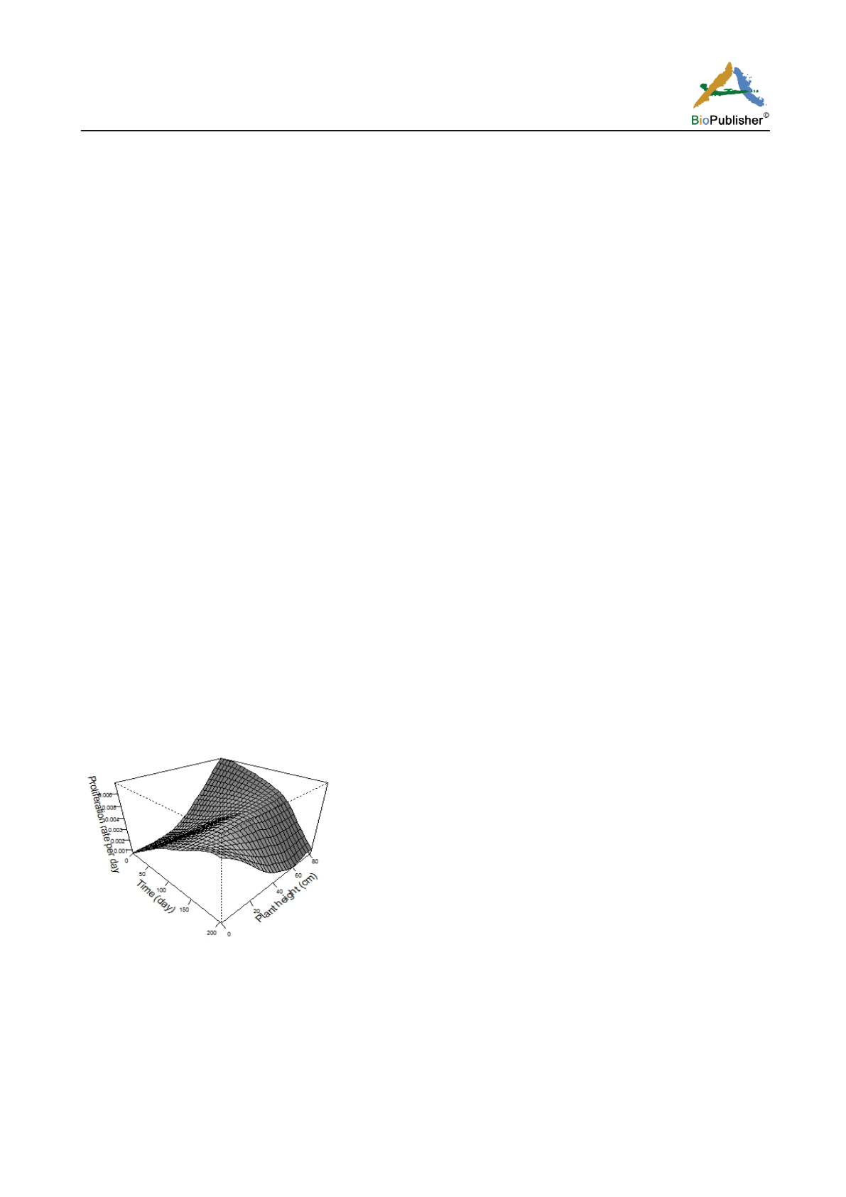
Figure 12 Proliferation rate of yield vs. time & plant height: 2nd interim cut
In a similar manner of drawing Figure 11, we draw Figure 12. Recall the set of time points considered in
constructing Figure 11 where at least one yield data is recorded. Over these time points, we consider plant height
for a fixed seed weight. There are height records at first interim growth recording time, second interim time, and
the last height on plant maturity. In total there are at least 5 observations on height recorded for each plant. The
set of time points considered for plant height recording is larger than that of underground yield, as height is an


